Architecture
The user perspective of mesh–generation packages is centred around specification of two parts: domain geometry and mesh element size.
Encoding domain geometry and mesh element size is a useful paradigm for describing meshes for large–scale geophysical modelling [Gorman_et_al:2006], as it organises the necessary information in a conceptually clear way.
We here follow the conventional norm in ocean modelling, discussed in the Introduction , where meshes are produced in a topologically two–dimensional space [Gorman_et_al:2006] and the domain is bound by various contours, typically topographic contours, and arbitrary lines.
The two primary data structures of GIS are used to describe linear features and field data.
A vector data structure can represent points, lines and regions on a reference surface, while a raster data structure encapsulates the discrete representation of fields.
The analogue to the abstraction used to drive mesh generators is clear: the domain geometry can be described with a vector data structure, while a raster can express the element size metric.
Thus, the obvious route to interfacing mesh generators with GIS is to provide a translation of GIS data structures into the corresponding structures native to the mesh generator software.
The data structure translation is at the heart of the qmesh package.
The translation is done with little user intervention, as the user typically interacts with the GIS package and parts of the qmesh package that facilitate specification of domain geometry and mesh element size.
To meet the demands around data archiving, publication and reproducibility a Research Data Management (RDM) tool is included in the qmesh package.
The RDM tool facilitates the process of publishing all resources, including output such as the mesh, to online, persistent and citable repositories.
The GIS package chosen is QGIS [QGIS_software], the mesh generator is Gmsh [Geuzaine2009-dd] and the PyRDM software library [Jacobs_etal:2014] was used to integrate research data management [Jacobs_etal:2015].
The main reasons for choosing QGIS, Gmsh and PyRDM, are robustness, extensibility and permissive licences.
Specifically, Gmsh is a robust mesh generator featuring a CAD–CAM interface, and has been used for generating meshes in various scientific and engineering domains, including geophysical domains [lambrechts_et_al:2008][Geuzaine2009-dd].
QGIS is a widely used GIS platform, with an active community of users and developers, and has been used as a user interface to mesh generation in past efforts [heinzer:2012][prodanovic:2015].
The functionality of QGIS is available to the user as a standard GIS system with a rich graphical interface and as an object–oriented Python module.
Therefore, QGIS is a solid framework on which to develop complex applications that require GIS methods.
Also, QGIS provides a framework for using such applications as extensions, via the QGIS graphical user interface.
Finally, QGIS, Gmsh and PyRDM are released under the GNU General Public Licence, making possible the use of qmesh in an academic or industrial context, free of charge.
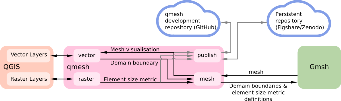
Fig. 1 presents an overview of the architecture of qmesh and conveys the usual work–flow.
As shown, qmesh is composed of four modules, named vector, raster, mesh and publish.
The purpose of the modules vector and raster is to facilitate the definition of the domain geometry and mesh–size metric and to interface qmesh to QGIS.
The translation between GIS and mesh–generator data structures is performed by the mesh module, thus interfacing qmesh to Gmsh.
The RDM functionality is implemented by the publish module, interfacing qmesh to online repositories and enabling identification and publication of data.
Apart from just conceptual, the modules shown in Fig. 1 are also the Python modules of the qmesh implementation and are discussed in detail in section Module design and implementation.
To allow access to the qmesh modules from a variety of environments three different User Interfaces have been developed, discussed in The qmesh interfaces and packages.
The interfaces are implemented as separate Python packages, to facilitate distribution, installation and namespace organisation.
The qmesh interfaces and packages
qmesh can be used in a graphical as well as a programmatic environment, through three different user interfaces:
- A Python–based Application Programming Interface (API).
- A Linux Terminal Command Line Interface (CLI).
- A Graphical User Interface (GUI).
Each interface is implemented as a separate Python package.
We have avoided the creation of a single monolithic package to minimise dependencies, to orthogonalize the module definition to the User-Interface definition (to the extent possible), but also to more narrowly define the purpose of each package and thus help in more targeted testing.
Thus, the following packages compose what collectively can be identified as qmesh:
qmesh. This is the “core” qmesh package, other APIs/packages require the qmesh package as a dependency.
According to the Python documentation, Python packages are a way of structuring the Python module namespace by using dotted module names.
Thus, the package presents a Python API and contains the implementation of the modules shown in Fig. 1, accessible as qmesh.vector, qmesh.raster, qmesh.mesh and qmesh.publish.qmesh-cli. This package contains the code needed to access the qmesh functionality from a linux terminal.qmesh-qgis-plugins. This package contains the code necessary to access the qmesh functionality from within QGIS, using a graphical interface.
Application Programming Interface
The Python-based API is an integral part of the qmesh implementation.
It can be used to build scripts that automate series of operations, but its primary purpose is to allow the use of qmesh as a software library.
It is the most powerfull and flexible of the qmesh interfaces, due to the power and flexibility of Python, its interactive shells (e.g. [PER-GRA:2007]) and numerous extensions.
Command Line Interface
The command line interface consists of a set of utilities each with well–defined input and output, making each utility a separate program.
However, their purpose is to be used as diagnostic tools or, to automate operations which do not require a graphical interface.
Graphical User Interface
The graphical user interface is a QGIS extension.
This way qmesh can be used via the QGIS application and in combination with other QGIS functionality.
The GUI has been designed to allow access to the qmesh package with ease and little knowledge of the qmesh design.
Module design and implementation
The qmesh implementation follows the object-oriented programming paradigm.
Thus, each of the modules shown in Fig. 1 contain class definitions that facilitate the aim of the module.
In this section, we describe the modules in more detail and summarise the classes typically used.
A complete listing of all definitions in each module can be found in the API Rerefence.
The vector module
The vector module is used to construct a complete definition of the domain geometry in terms of domain boundaries (lines) and domain surfaces (areas).
Surfaces are defined in terms of lines, so the definition of surfaces is automated by methods in the vector module such that only the boundary lines need to be supplied.
Other methods allow for essential geometric operations such as checking for erroneous geometries (i.e. intersecting shorelines) or the removal of small islands and lakes, based on a threshold surface area specified by the user.
The necessity of shoreline processing in ocean modelling is discussed in [Gorman_et_al:2008], where the Terreno project used GMT [Wessel_Walter:1991] to affect shoreline processing.
In qmesh however, geometry processing is done primarily through the QGIS software library, also allowing use of extensive functionality built-into the GIS platform.
In addition to geometry definition, methods for identifying separate parts of the domain geometry are necessary.
For example, open boundaries are associated with different boundary conditions to shorelines.
The qmesh user can assign numerical identifiers to separate lines and apply different boundary conditions to separate boundaries.
Numerical IDs can also be assigned to surfaces, allowing the identification of areas where different numerical treatments or parameterizations must be applied, as shown in the Tutorials.
The QGIS library is used to store and retrieve the digital IDs as standardised feature attributes.
The output of the vector module uses the ESRI shapefile [esri:1998] vector data–structure, which also supports storage of the ID feature attributes.
This way the module output as well as IDs can be visualised, assigned and edited with any GIS platform.
The raster module
The aim of the raster module is to facilitate construction of raster fields that describe the desired element edge length
distribution over the domain. For example, the element size might be chosen to be smaller in areas of shallow water, steep bathymetry and areas of
significant variation in bathymetry slope. Therefore an optimal element size distribution is typically expressed as a function
of bathymetry, its gradient and Hessian and the distance to boundaries [legrand_et_al:2000][legrand:2007][lambrechts_et_al:2008].
The raster module facilitates application of various mathematical operators to be applied to raster data such as derivatives, methods
for combining raster fields such as pointwise minimum and maximum operators, but also methods for calculating the distance function raster from
any given vector feature. The latter is useful when specifying a mesh size gradation towards specific features in
the domain: for example, the element size gradually becoming smaller as a coastline or a tidal turbine is approached. A generic method
has been implemented, aimed towards the construction of element size raster fields based on the distance from a given
vector feature (lines, polygons or points). This kind of operation is expressed by the arrows between the raster
and vector modules inside qmesh, in Fig. 1. As with the vector module, the output
of the raster module uses GIS raster data structures enabling visualisation and editing of the output via the GIS system.
The mesh module
The mesh module is used to translate the domain and mesh element size definitions into Gmsh data structures and,
as suggested in figure Fig. 1 can be used to convert the mesh into a vector data–structure.
Such functionality enables mesh visualisation using QGIS, and in particular to over–lay the mesh on other data. Various qualities
of the mesh can thus be assessed and the work–flow can be restarted towards improving the mesh.
The meshing module also allows the user to specify the coordinate reference system of the output mesh, which need not
be the same as that of the domain geometry and mesh–metric raster. Coordinates are reprojected to the
target coordinate reference system before the data is passed to the mesh generator. The reprojection procedure
uses the QGIS library; this way meshes can be obtained in all cartographic projections that QGIS supports and identifies
via an EPSG code. The output mesh is two–dimensional and the EPSG specification describes the dimensions,
including their units.
As a particular case, the output mesh can be constructed in a three–dimensional space, where the mesh vertices lie on a sphere, using specific Gmsh functionality described in [lambrechts_et_al:2008][remacle:2016].
The vertex coordinates are specified in terms of a Cartesian reference system whose origin lies at the sphere centre, the z–axis is the axis of rotation and the x–axis intersects the surface of the sphere at 0o longitude and 0o latitude.
Meshes thus constructed can be used to perform global simulations or simulations over large areas [Gorman_et_al:2006][lambrechts_et_al:2008][wells_et_al:2010][mitchell_et_al:2011][hill:2014][remacle:2016].
The publish module
The aim of the publish module is to facilitate provenance description and reproducibility of qmesh output.
Broadly, the specific version of qmesh used to produce the mesh and all of the input data sources are stored in an online repository.
In general data provenance may seem intractable since data and software are often stored in a non–persistent way and are not easily accessible.
However, given the increasing importance of data provenance, online data repositories with efficient storage and access controls such as Zenodo and figshare, are becoming popular means of archiving and dissemination.
Also, such services incorporate meta–data as means of describing hosted data and minting a unique Digital Object Identifier (DOI).
The DOI is a standardised [ISO26324:2012] citable identifier and is aimed to be assigned to digital objects, stored in a persistent way in open repositories.
Therefore, DOI is a widely–adopted identifier for digitally stored data, be that a scientific publication, the output of scientific computations or records from experiments and observations.
Given the wide range of data sources that can be combined during mesh generation for realistic geophysical domains, the task of manually maintaining the provenance information of all the relevant data files can be time–consuming and error–prone.
As shown in figure Fig. 1 the publish module interfaces with the qmesh development repository, via PyRDM [Jacobs_etal:2014][Jacobs_etal:2015], to identify the exact version of qmesh used.
A query is then made with the repository hosting service to establish if this version of qmesh has already been uploaded and assigned a DOI.
A similar query is performed for each input data source.
Each unpublished item is then uploaded and a new DOI is minted and assigned to the entire dataset.
The dataset also includes citations, in the form of meta–data, of the DOI markers of already published items.
The various DOI markers can be thought of as nodes of a tree, and the citations are the tree connections, a similar concept to scientific publications.
Also, the output can be archived in a private repository, without a DOI, to facilitate archival of commercially sensitive information.
| [1] | (1, 2, 3) G J Gorman, M D Piggott, C C Pain, C R E de Oliveira, A P Umpleby, and A J H Goddard. Optimisation based bathymetry approximation through constrained unstructured mesh adaptivity. Ocean Model., 12(3–4):436–452, 2006. |
| [2] | QGIS Development Team. QGIS Geographic Information System. Open Source Geospatial Foundation, 2009. URL: http://qgis.osgeo.org. |
| [3] | (1, 2) Christophe Geuzaine and Jean-François Remacle. Gmsh: A 3–D finite element mesh generator with built-in pre- and post-processing facilities. International Journal of Numerical Methods in Engineering, 79(11):1309–1331, 2009. doi:10.1002/nme.2579. |
| [4] | (1, 2) Christian T Jacobs, Alexandros Avdis, Gerard J Gorman, and Matthew D Piggott. PyRDM: A Python-based library for automating the management and online publication of scientific software and data. Journal of Open Research Software, 2(1):e28, 2014. doi:10.5334/jors.bj. |
| [5] | (1, 2) C. T. Jacobs, A. Avdis, S. L. Mouradian, and M. D. Piggott. Integrating Research Data Management into Geographical Information Systems. In Proceedings of the 5th International Workshop on Semantic Digital Archives. 2015. URL: http://hdl.handle.net/10044/1/28557. |
| [6] | (1, 2, 3, 4) Jonathan Lambrechts, Richard Comblen, Vincent Legat, Christophe Geuzaine, and Jean-François Remacle. Multiscale mesh generation on the sphere. Ocean Dynamics, 58(5-6):461–473, 8 October 2008. |
| [7] | Thomas J Heinzer, M Diane Williams, Emin C Dogrul, Tariq N Kadir, Charles F Brush, and Francis I Chung. Implementation of a feature-constraint mesh generation algorithm within a GIS. Comput. Geosci., 49:46–52, December 2012. |
| [8] | Pat Prodanovic. QGIS as a pre-and post-processor for TELEMAC: mesh generation and output visualization. In 22nd TELEMAC-MASCARET User Conference. 15 October 2015. |
| [10] | G J Gorman, M Piggott, M R Wells, C C Pain, and P A Allison. A systematic approach to unstructured mesh generation for ocean modelling using GMT and terreno. Computers and Geosciences, 34(12):1721–1731, December 2008. |
| [11] | Paul Wessel and Walter H F Smith. Free software helps map and display data. Eos Transactions AGU, 72(41):441–446, 1991. |
| [12] | ESRI. ESRI shapefile technical description. Technical Report J-7855, Environmental Systems Research Institute, July 1998. |
| [13] | S Legrand, V Legat, and E Deleersnijder. Delaunay mesh generation for an unstructured–grid ocean general circulation model. Ocean Modelling, 2(1–2):17–28, 2000. |
| [14] | Sébastien Legrand, Eric Deleersnijder, Eric Delhez, and Vincent Legat. Unstructured, anisotropic mesh generation for the northwestern european continental shelf, the continental slope and the neighbouring ocean. Continental Shelf Research, 27(9):1344–1356, 15 May 2007. |
| [15] | (1, 2) Jean-François Remacle and Jonathan Lambrechts. Fast and Robust Mesh Generation on the Sphere–Application to Coastal Domains. Procedia Engineering, 163:20–32, 2016. |
| [16] | Matrin R Wells, Peter A Allison, Matthew D Piggott, Gary J Hampson, Christopher C Pain, and Gerard J Gorman. Tidal modelling of an ancient tide-dominated seaway, Part 1: Model validation and application to global Cretaceous (Aptian) tides. Journal of Sedimentary Research, 80:393–410, 2010. doi:10.2110/jsr.2010.044. |
| [17] | Andrew J Mitchell, Peter A Allison, Gerald J Gorman, Matthew D Piggott, and Christopher C Pain. Tidal calculation in an ancient epicontinental sea: The Early Jurassic Laurasian Seaway. Geology, 39(3):207–210, 2011. doi:10.1130/G31496.1. |
| [18] | Jon Hill, Gareth S Collins, Alexandros Avdis, Stephan C Kramer, and Matthew D Piggott. How does multiscale modelling and inclusion of realistic palaeobathymetry affect numerical simulation of the Storegga Slide tsunami? Ocean Modelling, 83:11–25, 2014. doi:10.1016/j.ocemod.2014.08.007. |
| [19] | Technical Committee ISO/TC 46 (Information and documentation), Subcommittee SC 9 (Identification and description). ISO 26324:2012 Information and documentation – Digital object identifier system. Technical Report, International Organisation for Standardization, 2012. |